Contents
- Index
- Previous
- Next
Similarity/Diversity plotting
This is a good first step to cover, because it is faster and more intuitive than bootscanning. The results don't look as dramatic as bootscanning, but that is why similarity/diversity plots are more intuitive: in similarity/diversity plots one can see how similar/different two sequences are, not just how much more related they are to each other than to the other sequences/groups being compared (i.e. absolute versus relative similarity). An example of this sort of confusion is demonstrated on the Pitfalls page.
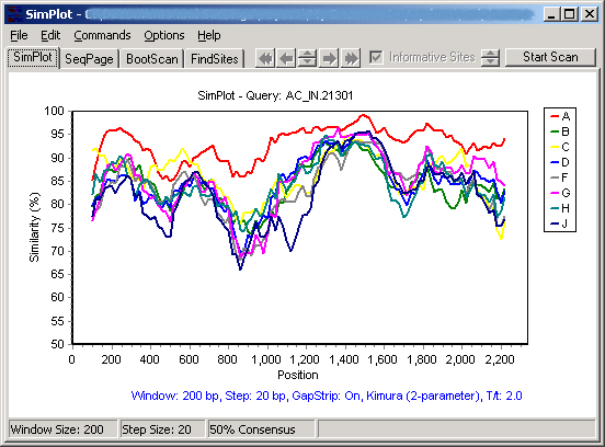
First, click on the "SimPlot" tab (next to the "SeqPage" tab) to flip to the chart that's used to plot similarity and diversity. Use the Commands menu to select a query group, then go again to the Commands menu and select "Do SimPlot". If you have not altered any of the options, this will generate a similarity plot using the 2-parameter (Kimura) distance model, in a sliding window of 200 nucleotides, step size of 20. It will look something like this:
Clicking on the Y axis (on the left) will allow selection from a number of options. From the same plot, selecting diversity plot and decimal display results in the following diversity plot:
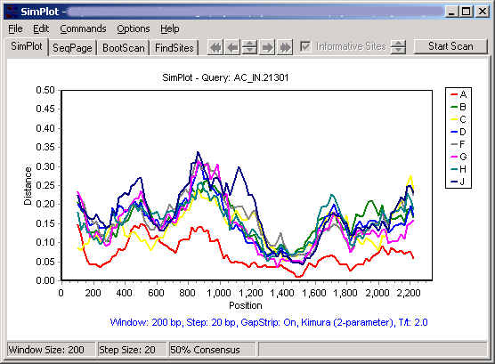
Note that the plots appear to be missing about 100 residues at each end - this is because each point is placed at the midpoint of the window it represents. These gaps will always be 1/2 the window size.
To adjust the Window size or Step size, just click on them and choose a new value:
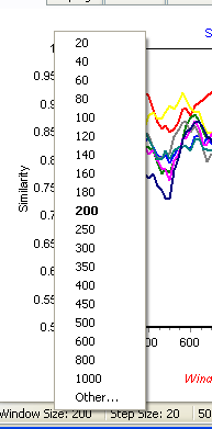
Larger window sizes will tend to flatten the curves, increasing accuracy of distance measurements but reducing the likelihood of observing evidence for small recombinant segments.
Smaller step sizes add more detail by adding more data points, and thus plots with small step sizes take longer.
Note: The raw values of the plots can be saved in comma-delimited format from the File menu.